Why and how I built a SQL Join tool for Alteryx Designer
by Nathan Purvis
Background
For anyone who may not have a clue what I’m talking about when I say the SQL Join tool for Alteryx Designer, I recently announced the release of my latest custom macro on LinkedIn, the post for which you can find here.
Follow this link to download.
Follow this link for the supplementary information.
So what is it? Well, for anyone familiar with Alteryx Designer, you’ll know that the current, native Join tool only allows you to conduct strict, like-for-like blending i.e. ‘table1.A = table2.A’. There isn’t any support for other operands or join conditions like we see in SQL such as ‘table1.A <= table2.A’ or ‘table1.A BETWEEN table2.A AND table2.B’. After noticing this and seeing a couple of posts on the Alteryx community highlighting this as a pain point, I decided to think about how I could build a solution that accommodates more flexible blending within Alteryx Designer. I also wanted to ensure that this didn’t involve using a) the Append Fields tool (which creates a cartesian product), or b) the Generate Rows tool (i.e. forming a scaffold across ranges which we can then join on). Why? Simple - both of these methods lead to a blow up in the volume of our dataset(s) which is generally bad practice if we can avoid doing so.
The workflow
I’ll outline each stage of the workflow before and how it works, but here’s a high-level image of it beforehand:

To start with, we obviously need our Macro Inputs - these take in the left and right data streams in the exact same way as the native Join tool. A RecordID is added to each feed in order to conduct the left and right joins in the final stages of the macro which we’ll see further on in this blog. After assigning a RecordID, a prefix of ‘R_’ is assigned to all fields coming in via the right-hand side; this is to prevent errors from ambiguous field names (identical field names existing in both the left and right table) when the SQL query is executed. The final part of this initial stage is then writing both of these streams to temporary In-DB tables. This allows us to load our data into a database so that we can then query it using SQL to provide the added flexibility we’re looking for in the join clause. Making the tables temporary also has an added benefit in that they will only persist for the duration of the macro run, meaning you don’t need to worry about constantly storing two additional tables. The image below isolates the section that we’ve just covered, in case you’re struggling to follow!

Now that we have the two (left and right) starting datasets loaded into our database, we can execute our query. However, we first need to create this and, in order to do so, we need two things: to find the names of these tables (which are always changing as they’re temporary and named automatically by Alteryx), and our join clause. That’s what this section handles:

So what’s going on here? The wireless connection you see feeding into the initial Filter tool comes from the Control Container holding the two Data Stream In tools from our first section. One of the great functionalities of Control Containers is that we can print workflow messages as data. Therefore, we’re essentially creating a dataset here that is made up of the previous part’s event logs. When the temporary tables are created, we get very clear messages which we can isolate through the Filter, like so:

Once these messages are separated from the others, we need to sort by ToolID which ensures the record holding the message from the left table is above the right - if one table is larger than the other then they will inevitably take longer to write into the DB and so sometimes the right-hand message will print first and appear above the left in the workflow messages. This sorting step is crucial because of the step after the Formula tool where records are concatenated in the order they appear. Following the sort, we just use some simple string functions to look for the quotation marks that hold the table name and parse a substring from this. Then, as mentioned just now, we use a Summarize tool to concatenate the two table names, using ‘ JOIN ‘ as a separator. The result is our [Concat_TableNames] field which looks like ‘LeftTable JOIN RightTable’. For this section, the penultimate step is appending a Text Input to our data. This tool holds our join clause and as a default is set to ‘ ON 1=2’, so that if no end-user input is provided, no join will occur. We’ll see later on that an interface tool is set to replace the ‘1=2’ part with the user entry. So now that we have ‘LeftTable JOIN RightTable’ and ‘ ON <condition>’, the only thing left is to select columns, which we do in the final tool of this section - the Formula. In here, the first expression adds ‘SELECT * FROM’ to the [Concat_TableNames] and [User Input] fields, resulting in our final custom query i.e. ‘SELECT * FROM LeftTable JOIN RightTable ON <condition>’. A second expression then just prints a string of the connection name which is needed to feed into the Dynamic Input In-DB tool. Once more, this field is updated by an interface tool that replaces the <Dummy Connection Name> value with the user’s value.
The third section of the macro is where the join actually happens - using the query built as detailed above, along with the connection name, we run both of these through the Dynamic Input In-DB tool and then use a Data Stream Out tool to get the resulting dataset from the DB into our workflow. You’ll also notice a wireless connection on the Control Container itself. This is linked to the output of the first Control Container (where the two temporary tables are created) and ensures that that has finished before trying to execute the query. The image below shows this workflow stage:

We now come to the final processing part of the workflow, as the only other remaining part - which will be covered last - handles all of the interface tools. That looks like this:

This section pretty much just cleans things up ready for output to the main workflow. The first step here is a Dynamic Rename tool that strips the ‘R_’ prefix we needed to add to prevent ambiguous field name errors. Following that, we conduct two joins with the incoming data, using the temporary RecordID we assigned at the start of the macro as our key values; this allows us to see left and right join products and present all three outputs to the end-user, instead of just the inner join product. Finally, just before our Macro Output tools, we simply sort on the temporary left and right RecordID fields so that records come out in ascending order, before using a Select tool to remove these columns.
Finally, we just need to cover our interface tool section i.e. the part of our workflow that handles user-input and feeds this into the necessary tools:
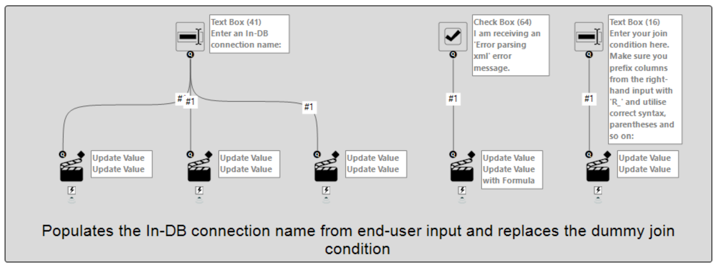
Working from left to right, we first have an initial Text Box which prompts the user to input their In-DB connection name. This is needed to populate the configurations of the two Data Stream In tools, as well as the Dynamic Input In-DB tool. Second up is the Text Box that the user can tick if they are receiving an error about XML parsing. In the Action tool a formula expression is used so that, if the box is checked, special XML characters in the join clause i.e. < and > will be replaced with < and > respectively in order to try and avoid this. The third and final interface tool is another Text Box which asks the user to provide their actual join clause, replacing the dummy ‘1=2’ value.
…and that’s a wrap on the breakdown of this macro! I had a lot of fun building this out as a proof of concept and overcoming the range of obstacles that crept up throughout testing. Hopefully you can take the time to check it out and find some use for it, of course adjusting it as necessary for your own use-case! As usual, please reach out with any questions, feedback or requests for future tooling and content.